Using simple linear regression for BLS estimate

The following post will explore using LinkUp’s data to make a simple prediction for nonfarm, non-seasonal total employment numbers using linear regression. The intention is not to create a perfect prediction in this tutorial, but to iterate on this model in subsequent posts and show possible methods of engineering LinkUp’s data to improve our prediction as the Bureau of Labor Statistics (BLS) releases new monthly jobs numbers. If you are looking for a tested and perfected prediction I would suggest turning to the latest blog post by our CEO, Toby Dayton. All of the work can be done in Excel, but we will be using Python for enhanced charting capabilities. For simplicity sake, very little filtering or cleaning of LinkUp’s data will be done for this post.

The two datasets that will be used here are: all job listings in LinkUp’s database with U.S. listed as the location, and the CES total nonfarm, non-seasonally adjusted dataset from BLS found here. Of note, BLS revises its employment numbers 3 times; we will be using the revised numbers, apart from the 2 most recent months numbers, since they have yet to be revised.

First we will prepare our LinkUp dataset, which can be done in a few different ways. We can filter down the raw dataset to only include jobs postings with ‘U.S.’ as the country field, or we can take a pre-aggregated report and use that. For this we will take the simpler route and use the aggregated report for active jobs by states and month, and sum them to get a U.S. total. This is ideal for users who are not interested in dealing with the large, raw full dataset, or for users looking for a quick series to test. The raw dataset offers far more possibilities in terms of the series we can create, for example filtering out all farm related O*NET codes. In later posts we will see how moving from the pre-aggregated series to raw data can lead to more options.

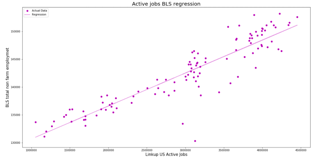
Now that we have our 2 datasets we should check to see that they share some type of relationship.

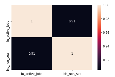
There looks to be a linear relationship between our independent and dependent variables. We can further explore this by looking at the correlation between our variables.

Now that we have established the relationship we can build the model. Below is our regression line in red, with the actual data scattered in blue points.

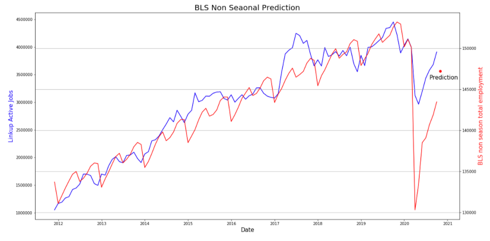
With our model built we can feed in our active job data from October to get a prediction of 147,205. Up from BLS’ last reported number of 143,459.

While this was a good start, and shows the predictive possibilities LinkUp’s data can offer, there are some assumptions that should be accounted for.

Both of these datasets show high autocorrelation
Both of these datasets appear to be Gaussian-like in distribution
Our BLS data incorporates revision and is not point in time, creating a look ahead bias
Our LinkUp data incorporates drift, also factoring in look ahead bias
The LinkUp sample size is always growing due to our continually expanding coverage

The above assumptions all have an effect on the accuracy of our prediction. In our next tutorial dealing with prediction, we will work with our 2 datasets to account for these assumptions mainly by using raw data to filter the LinkUp dataset.